Zero-knowledge proofs (ZKPs) allow a party to prove a statement to another party without revealing any additional information beyond that the statement is true. Though this cryptographic primitive has existed since the 1980s, it wasn’t until the emergence of blockchain technology that ZKPs found practical applications including blockchain scalability, privacy, interoperability, and identity.

Despite its promise of solving many of the biggest issues in blockchain technology, ZK remains an immature technology. Among its major issues is its long proving times. As ZK applications have advanced, so have the complexity of their proofs. These statements require larger arithmetic circuits, driving up proving times. Producing a ZKP can require up to a 1,000,000x increase over the underlying computation. Consequently, a number of teams are researching methods to improve the software and hardware needed to accelerate ZKPs.

In this article, we provide an overview of ZKP acceleration. We begin with a summary of the main operations in ZKP generation, then turn to how these operations can be accelerated.

Introduction to Zero-Knowledge Proofs

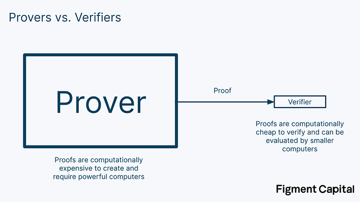
ZKPs allow one party, called a prover, to prove to another party, called a verifier, that they correctly performed a computation. A ZKP system has 3 key properties:

• Completeness: If the prover generates a valid proof, an honest verifier will conclude that the statement is valid.
• Soundness: If the statement is false, a prover will not be able to generate a proof that looks valid.
• Zero-knowledge: If the statement is true, a verifier does not learn anything beyond that it is true.

The main type of ZKPs used in the blockchain context are zk-SNARKs (or “zero-knowledge succinct non-interactive arguments of knowledge”). These proofs add 2 additional properties to traditional ZKPs: succinctness and non-interactivity. Having succinctness means that the proof size is small, often just a few hundred bytes, and can quickly be checked by the verifier. Non-interactivity means that the prover and verifier don’t need to interact; the proof itself is enough. Older ZKPs required provers and verifiers to send messages back and forth to generate a proof.

Succinctness makes ZKPs quick and computationally cheap to verify. This makes them an excellent scaling technology. In validity rollups (i.e. zkRollups), powerful provers can compute the output of many thousands of transactions, produce a succinct proof of their correctness, and send them to the base chain. There, verifiers can check the proof and immediately accept the results of all included transactions without having to compute them themselves. Thus, the network can scale while the base chain remains decentralized.

Packing thousands of transactions into a single proof requires a tremendous amount of computation and results in long proving times. Long proving times create longer times to finality as users’ transactions do not have full finality until their transaction and its proof have been submitted to the base chain. This can take a while. In Starknet for example, we anticipate proving times will initially take several hours. ZKPs need to be accelerated for better performance, security, and UX.

A ZKP system has 3 steps: setup, proof generation, and proof verification.

There are 6 values used in the proof.

• R - Random number: A one-time secret random number is needed to set up the ZKP system. If any party knows the random number, they can break the code and identify the secret input value, eliminating the zero-knowledge property. This is where the idea of “trusted setups” comes from. In trusted setups, many parties come together to collectively generate the random number such that no individual learns the secret. As a user, you must trust that the setup was done correctly (i.e. that nobody knows R), for your information to stay private. Note that STARKs do not require trusted setups.
• Sₚ - Prover setup parameters: Parameters given to the prover after the setup that allow it to generate a valid proof.
• Sᵥ - Verifier setup parameters: Parameters given to the verifier after the setup that allow it to verify a valid proof
• X - Public input values: The input values we use to perform the computation. These are given to both the prover and the verifier and are not a secret.
• W - Private input value: This is the secret input value, called a witness, given only to the prover. Notice in the diagram above that the witness is not passed to the verifier. The essence of ZK is that it enables us to prove statements about the witness without needing to reveal it.
• P - The Proof: This is the proof created by the prover and sent to the verifier.

That is zero-knowledge in a nutshell. That’s it! When you look at it, it’s actually fairly simple. But to understand how to accelerate ZKPs, we must understand how they work under the hood.

MSMs and NTTs

There are two main bottlenecks in ZKP generation: Multi-scalar Multiplications (MSMs) and Number Theoretic Transforms (NTTs). These operations alone can account for 80–95% of the proof generation time, depending on the ZKP’s commitment scheme and specific implementation. First, we’ll introduce these operations, then we’ll provide an overview of how each can be accelerated.

Prime Finite Fields

Let’s start with prime finite fields. Both MSMs and NTTs occur within prime finite fields, so understanding them is an important first step.

Imagine we have a set of numbers 0–10. We can add a rule to this set of numbers that says: once we count past the number 10, we start back at the number 0. For example, if we add 9+2=11, we would loop back to the beginning of the set to get 0. Subtraction works similarly. If we subtract past our lowest number 0, we start back at the end with 10.

We call the number 11 the modulus since it’s the number at which we “loop around.” This type of math is called modular arithmetic. Our most intuitive experience interacting with modular arithmetic is in telling time, where we count our hours modulo 12.

Multiplication also works in modular arithmetic. If we take 9*3=27, we would get 5 as our output (count for yourself if you’d like to check!). This is called the “remainder” in simple division. We could write the solution as:

9 * 3mod(11) = 27mod(11) = 5, since 11*2 + 5 = 27. The 2 represents the number of times we looped around the set.

Notice that in our set of 0–10, no matter what numbers we choose for addition, subtraction, or multiplication, our result will always be another number in the set. In other words, there’s no way to break out of the set. Division is slightly more complicated in modular arithmetic, but it works similarly. Because our set has this closed nature, it is a special type of set called a field.

Going from a field to a prime finite field is trivial. A finite field is a field with a finite number of elements in it. A prime finite field is a finite field that has a prime number as its modulus. Since our example set of 0–10 is finite and has the prime number of 11 as its modulus, it’s a prime finite field!

Multi-scalar Multiplications

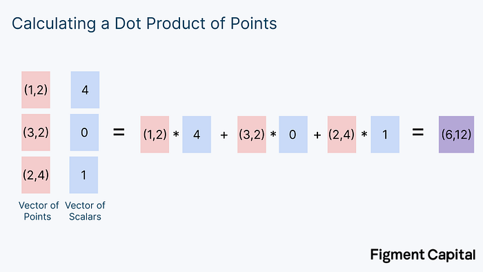
Now that we’ve covered prime finite fields, we’re able to understand MSMs. Say we have 2 rows of numbers. One operation we could perform on these rows is to take each element in a row, multiply it with its corresponding element in the other row, and add the products up into a single number. This operation is called a dot product, and is commonly used in mathematics. Here’s what it looks like:

A vector is just a list of numbers. Notice that we took 2 vectors of numbers as input, and produced a single number as output. Now, let’s modify our example. Instead of calculating the dot product of 2 vectors of numbers, we could calculate the dot product of a vector of points and a vector of numbers.

A scalar is just a normal number. In this case, our output isn’t an individual number, but a new point on a grid. Graphically, the calculation above looks like this:

This computation involves scaling each point on the grid by some factor, and then adding all the points together to get a new point. Notice that no matter what points on this grid we pick and no matter what scalars we multiply them by, our output will always be another point on the grid.

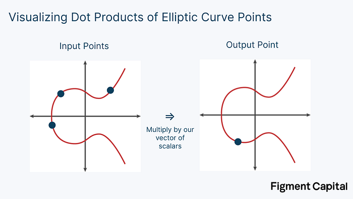
Just as we could calculate the dot product with points on a grid instead of integers, we could also perform this calculation with points on an elliptic curve. An elliptic curve (EC) looks like this:

The math we use in ZK involves elliptic curves that sit within prime finite fields. Therefore, no matter what addition or multiplication we perform on any point on the elliptic curve, its output will always be another point on the elliptic curve. The dot product of scalars will output another scalar, the dot product of (x,y) coordinates will produce another coordinate, and the dot product of elliptic curve points will produce another EC point. Visually, elliptic curve dot products look like this:

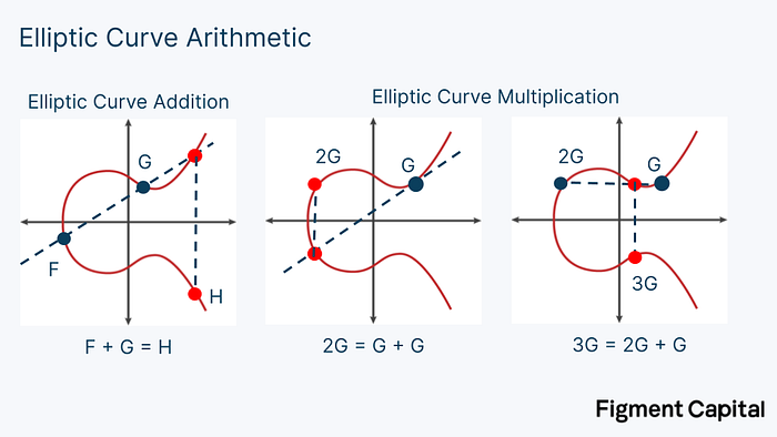
Multiplying a point on an elliptic curve by a scalar is called point multiplication. Adding two points together is called point addition. Both point multiplication and point addition output a new point on an elliptic curve.

Visually, elliptic curve addition is a simple operation. Given any two EC points, we can draw a line between them. If we look at where that line intersects the curve a third time, we can find its reflection over the x-axis to find the sum of the two points. To add a point G to itself, we find the tangent line to the curve, see where that line intersects with the curve, then draw a line reflecting on the x-axis until we intersect the curve again. That point is 2G. Therefore, point multiplication is also easily visualized. It merely involves adding up a point by itself.

A detailed explanation on how to calculate EC addition mathematically is beyond the scope of this article. At a high-level, EC addition takes two very large integers and adds them together, modulo some large prime number.

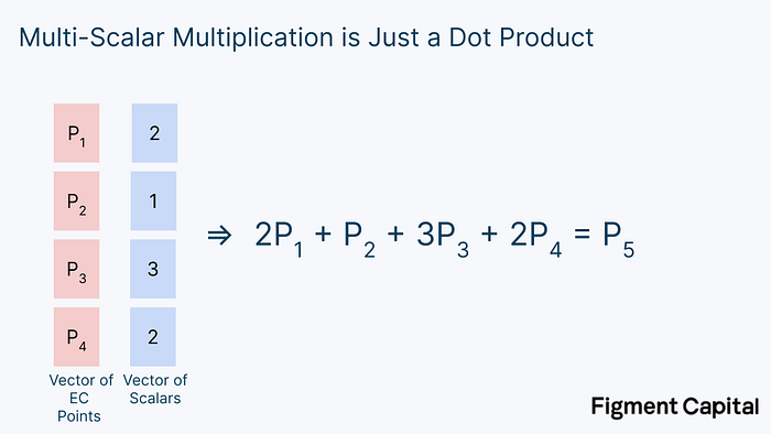
This operation of taking multiple elliptic curve points, multiplying them by scalars (point multiplication), and summing them (point addition) to get a new point on the elliptic curve is called Multi-scalar Multiplication (MSM). MSM is one of the most important operations in ZKP generation, yet it is just a dot product.

It’s actually even simpler than that: MSM can be rewritten as a bunch of EC point additions.

So whenever you hear “Multi-scalar Multiplication,” all we’re doing is adding many EC points together to get a new EC point.

The Bucket Method

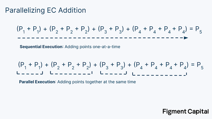
The “bucket method” is a clever trick used to accelerate MSM calculations. Point addition calculations are computationally cheap. The problem with MSMs are the point multiplications. In real ZK proofs, the scalars we are multiplying our EC points by are extremely large. For every point multiplication, the calculation will require millions of summations. Luckily, there’s an easy way to speed up MSMs: we can compute all of our point multiplications in parallel.

The key idea in the bucket method is that we can reduce these large dot products into smaller dot products, compute them in parallel, and then add them together.

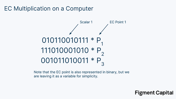
Here’s how it works. Recall that in a computer, numbers are represented as a binary number of 1s and 0s.

So on our computer, our EC multiplications might actually look something like this (only with much larger binary numbers):

The first step in the bucket method is to split these binary scalars into windows of a certain number of bits. In the image below, we segment the scalars into windows of 4 bits.

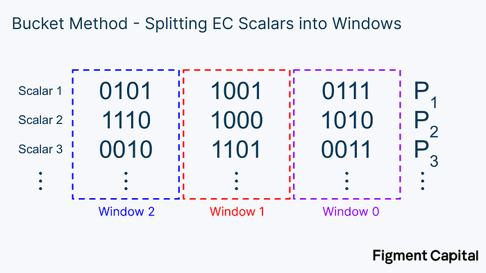
Notice each bucket covers values from 0000 = 0 to 1111 = 15. After we have broken our scalars down into windows of 4 bits, we can sort each EC point into buckets covering the range of 0–15.

For a given window, once we have sorted every point into a bucket, we can add all the points up to get a single point for each bucket.

Note that in this example we’re only showing a few points, but in practice, every bucket contains many numbers. Once we have each bucket value, we can multiply them all by their bucket number to get the final value of the entire window. This window calculation is just another dot product.

Once we have calculated the window value for each window, we can add them all up to get our final output. But first, we need to adjust for the fact that each of these windows represent different ranges of values. To do this, we need to multiply each window by 2ⁱ*ˢ, where i is the window number and s is the window length. Our windows are 4 bits long so the window size is 4.

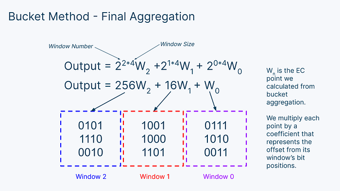
Then, we just add up all the numbers to get the final output of our MSM! To recap, the bucket method involves 3 steps: bucket accumulation, bucket aggregation, and window aggregation.

• Bucket Accumulation: For each window, sort each EC point into a bucket based on its coefficient. Then add up all the points in each bucket to get each final bucket value.
• Bucket Aggregation: For each window, multiply all the bucket values by their bucket number and add them together to get a window value.
• Final Aggregation: Take all the window values, multiply them by their bit offset, and add them all together to get your final elliptic curve point.

This bucket method is used in almost every ZKP acceleration setup. For example, below is a diagram of a hardware accelerator for MSM co-designed by the Jump Crypto and Jump Trading teams. Much of it looks familiar!

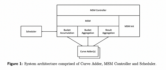
The bucket method accelerates MSMs by parallelizing the computation and effectively balancing the workload on hardware, leading to significant improvements in proof generation time.

Number Theoretic Transforms (NTTs)

NTTs, also referred to as Fast Fourier Transforms (FFTs), are the second key bottleneck in ZKP generation. The operation and underlying mathematics are more complex than MSMs, so we won’t provide a technical explanation here. Instead, we’ll touch on some intuition for how and why they’re computed.

ZKPs involve proving statements about polynomials. A polynomial is a function like f(x) = x² + 3x + 1. In ZKPs, the way that a prover demonstrates they have some secret information is by showing that they know an input to a given polynomial that evaluates to a given output. For example, the prover may be given the polynomial above, and tasked with finding an input that makes the output equal 11 (the answer is x = 2). Although this task is trivial for small polynomials, it becomes challenging when the given polynomial is very large. Indeed, the whole basis of the ZKP is that this task is so difficult for large polynomials that a prover will not be able to repeatedly find the answer unless they know the secret witness.

A necessary step then is to evaluate a polynomial to demonstrate that it equals a certain output. In ZK, these polynomials are represented by arithmetic circuits.

Arithmetic circuits take a vector of inputs and produce a polynomial evaluated at those points. The size of arithmetic circuits varies dramatically by application, ranging from ~10,000 to over 1,000,000.

We can straightforwardly evaluate a polynomial by inserting a number and calculating its output. Here’s an example:

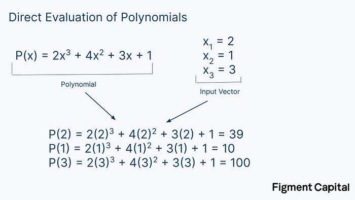
This method is called direct evaluation, and is how polynomials are typically evaluated. The problem is that direct evaluation is computationally expensive — it requires N² operations, where N is the degree of the polynomial. So while this is not a problem for small polynomials, direct evaluation becomes prohibitively large when dealing with large arithmetic circuits. NTTs solve this. By taking advantage of a pattern behind the evaluation of very large polynomials, NTTs can evaluate a polynomial with just N*log(N) computations.

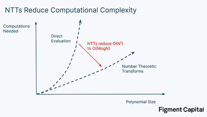
If we’re evaluating a polynomial with a degree of 1 million (meaning the highest exponent in the polynomial is 1 million), it would take 1 trillion operations to directly evaluate. Computing the same polynomial with NTT would take just 20 million operations — a 50,000x speed up.

In summary, evaluating polynomials plays a critical role in ZKP generation and NTTs allow us to evaluate polynomials more efficiently. However, even with this technique, the processing time of large NTTs remains a major bottleneck in ZKP generation.

ZK Hardware

We’ve given a high-level overview of the most important computations for ZKP acceleration. Algorithmic improvements like the bucket method for MSM and NTTs for evaluating polynomials led to major advancements in ZK proving times. But to improve ZKP performance even further, we must optimize the underlying hardware.

Accelerating MSMs and NTTs

As we demonstrated with the bucket method, MSMs are easily parallelizable. However, even when heavily parallelized, the compute time remains long. Moreover, MSMs have massive memory requirements that stem from needing to store all the EC values being operated on. So while MSMs have the potential to be accelerated on hardware, they require tremendous memory and parallel computation.

NTTs are less hardware friendly. Most importantly, they require frequent shuffling of data to and from external memory. The data is retrieved from memory with a random access pattern, which adds latency to the data transfer time. Random memory access and data shuffling becomes a major bottleneck and limits NTTs’ ability to be parallelized. Most of the work on accelerating NTT has focused on managing how the computation interacts with memory. For example, this paper from Jump describes a method to minimize memory access latency by reducing the number of times memory needs to be accessed and by streaming data to the computer chip, thereby accelerating NTTs.

The easiest way to solve the MSM and NTT bottlenecks is to eliminate the operation entirely. Indeed, some recent work like Hyperplonk introduces a modification to Plonk that removes the need to perform NTTs. This makes Hyperplonk simpler to accelerate, but introduces new bottlenecks like an expensive sumcheck protocol. On the other end of the spectrum, STARKs do not require MSMs, also providing a simpler optimization problem.

However, accelerating MSMs and NTTs is only the first step in ZK acceleration. Even if we could hypothetically drop the computation time of both MSMs and NTTs to 0, we would only achieve a 5–20x speed up in proof generation time. This is due to Amdahl’s law, which notes that acceleration is bounded by the fraction of time where we’re actually performing the computation. If MSMs and NTTs account for 90% of the proving time, eliminating them would still leave 10% of the proving time.

While speeding up MSMs and NTTs are important, they are just the start. To make further progress, we must also accelerate the “other” operations which include witness generation and hashing.

Hardware Overview

There are four main types of computer chips: CPUs, GPUs, FPGAs, and ASICs. Each chip has different tradeoffs in its architecture, performance, and generalizability.

Central Processing Units (CPUs) are the chips found in most consumer electronics like laptops. Their general-purpose nature makes them well suited for a wide range of devices and everyday tasks. High generalizability comes at the expense of performance. CPUs can only handle operations sequentially, making it perform poorly for many applications.

Graphics Processing Units (GPUs) are a more specialized chip. They have a large number of cores for parallel processing, making them especially suitable for applications like graphics rendering and machine learning. Although less general than the CPU and less specialized than the FPGA or ASIC, GPUs are a prevalent and accessible piece of hardware. Their popularity has led to the development of low-level libraries like CUDA and OpenCL that help developers take advantage of the GPUs parallelizability without needing to understand the underlying hardware.

Field Programmable Gate Arrays (FPGAs) are customizable chips that can be optimized for a given application in a reusable way. Developers can use Hardware Description Languages (HDLs) to program their hardware directly, enabling higher performance. The hardware can be modified repeatedly without the need for a new chip. The downside of FPGAs is their greater technical complexity — few developers have experience programming them. Even with the necessary expertise, research and development costs to customize FPGAs can be costly. Nonetheless, FPGAs have applications in industries ranging from defense tech to telecommunications.

Application-Specific Integrated Circuits (ASICs) are custom designed chips hyper-optimized for a specific task. Unlike an FPGA which allows for hardware reprogrammability, ASIC specifications are ingrained in the chip, preventing them from being repurposed. ASICs are the most powerful and energy-efficient chips for any given task. For example, Bitcoin mining is dominated by ASICs which compute far more hashes than any other type of chip.

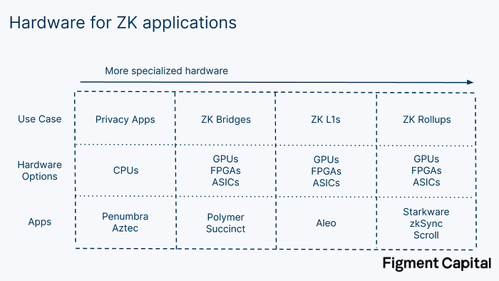
Given these options, which is best for ZKP generation? It depends on the application. Privacy apps like Penumbra and Aztec allow users to transact privately by creating a SNARK of their transactions before submitting to the network. Since the required proof is relatively small, it can be generated within their local browser just using their CPU. But for larger ZKPs that truly need hardware acceleration, CPUs are insufficient.

Hardware Acceleration

We can accelerate ZK proofs on hardware in a number of ways:

• Parallel processing: Performing independent computations at the same time
• Pipelining: Making sure that all our computer’s resources are being used at all times to maximize how much we can compute in a single clock cycle
• Overclocking: Increasing the clock speed of the hardware above the default speed in order to accelerate computations. This can damage the hardware if not done carefully.
• Increasing Memory Bandwidth: Using higher bandwidth memory to increase the speed at which we can read and write data to memory. In ZK, the bottleneck for proof generation is often not the computation, but the passing of data.
• Implementing better representations of big integers in memory: GPUs are designed to perform computations over floating-point numbers (i.e. decimal numbers). ZK operations are done over large integers in finite fields. Implementing a better representation of these large integers in memory can reduce memory requirements and data shuffling.
• Making memory access patterns predictable: Papers like PipeZK explore methods to make memory access patterns predictable while computing NTTs, making them easier to parallelize.

Any type of chip can be pipelined and overclocked. GPUs are well suited for parallelization, but their architecture is fixed; developers are limited to the cores and memory provided. GPUs cannot create better representations for big integers nor can they make memory access patterns more predictable. While GPU libraries such as CUDA and OpenCL offer some level of flexibility, the hardware has limitations; higher performance ultimately requires more flexible hardware. Nonetheless, GPUs can still accelerate ZKPs. Ingonyama, a ZK hardware acceleration company, is building ICICLE, a ZK acceleration library built in CUDA for Nvidia GPUs. The library contains tools to accelerate common ZK operations like MSMs and NTTs.

FPGAs have a lower clock speed than GPUs but can be programmed to address all the acceleration strategies above. Their biggest problem is just programming them. For ZK, organizing a team that has both the cryptographic expertise and the FPGA engineering expertise is extremely difficult. Early teams that have produced FPGAs for ZK acceleration have been sophisticated trading firms like Jump Crypto and Jane Street that already had FPGA and cryptography talent. FPGAs also still have bottlenecks — a single FPGA often doesn’t have enough on-chip memory to perform NTT, requiring additional external memory.

The most rigorous attempts to commercialize hardware-driven ZK acceleration are going even further than single FPGAs. For further gains, companies like Cysic and Ulvetanna are building FPGA servers and FPGA clusters that combine multiple FPGAs to provide additional memory and parallelizable compute to further accelerate proof generation. Early results from these teams are promising: Cysic claims their FPGA server is 100x faster at MSM than Jump’s FPGA architecture and 13x faster at NTT than the best known GPU implementation. Standardized benchmarks haven’t been established yet, but the results point to major improvement.

ASICs are able to provide the absolute highest performance for ZKP generation. The problem with ZK ASICs today is that they are optimizing for a moving target — ZK is rapidly developing. Since ASICs take 1–2 years and $10–20M to produce, they must wait until ZK has solidified enough that the chips produced don’t quickly become obsolete. Moveover, the market size of ZK proving is only becoming large enough to justify the capital investment needed for ASIC in the next couple years.

There’s a subtle gradient between FPGAs and ASICs. Though FPGAs are programmable, they have hardened parts of their chip that are not programmable. Solidified components have much higher performance than programmable ones. As the ZK market grows, FPGA companies like Xilinx (AMD) and Altera (Intel) could produce new FPGAs that embed hardened components specifically designed for common operations in ZK proving. Similarly, ASICs can be designed to include some flexibility. Cysic, for example, has future plans to produce ASICs that specifically target MSMs, NTTs, and other general operations, while maintaining flexibility to adapt to many proving systems.

In the long-run ASICs will provide the strongest ZKP acceleration. Until then, we expect FPGAs to serve the most computationally intensive ZK use cases, as their programmability enables them to perform NTT, MSM, and other cryptographic operations faster than GPUs. For some applications, GPUs will provide the most attractive balance between performance and accessibility.

Conclusion

The blockchain industry has spent years waiting for ZKPs to be production-ready. The technology has captured our imagination with promises of enhancing the scalability, privacy, and interoperability of decentralized applications. Until recently, the technology has been unrealistic, mainly due to hardware limitations and long proving times. This is rapidly changing: advancements in ZKP proving schemes and hardware are solving computational bottlenecks like MSMs and NTTs. With better algorithms and more powerful hardware, we can accelerate ZK proofs enough to unlock their potential to revolutionize Web3.

Acknowledgements: Special thanks to Brian Retford (RiscZero), Leo Fan (Cysic), Emanuele Cesena (Jump Crypto), Mikhail Komarov (=nil; Foundation), Anthony Rose (zkSync), Will Wolf and Luke Pearson (Polychain), and the Penumbra Labs team for great discussions and feedback which contributed to this piece.